Command-line measurements and acquisitions
Once the system and telescope setup had been completed, it is possible to manually perform measurements and observations through the TPB, which might as well pave the way – as preliminary checks – to longer lasting sessions carried out via schedules.
Raw counts readouts
The raw counts readout (called Tpi) of the signal can be obtained with:
> getTpi
The system reply consists in an array of values (one for each section). As concerns the TPB, it is important to ascertain that the Tpi lies within the 750-1000 counts range in order to keep your observations in the linear range of the backend and allow for fairly bright sources to stay within as well. If this requirement is not met, it is necessary to iteratively vary the attenuation for the needed sections and check the Tpi, until the signal intensity falls into the proper range.
As the signal level greatly varies with elevation, it is advisable to perform this operation in the elevation range that will be actually exploited during the observations or, as a general rule, at elevation=45°. Of course, the signal level is also greatly affected, especially at high frequencies, by weather conditions, therefore the attenuation tuning should be carried out again every time the conditions change.
When you are going to manually get the Tpi - in order to ascertain which attenuation values to use in your schedule - remember to set the LO frequency and the bandwidth as they will be employed in the schedule. After a setup command, in fact, they are set to defaults; instead, if a schedule has been previously run, these values remain set as indicated in the last schedule readout.
Note
Tpi values include the Tp0 level (the internal, “without sky” level, which is roughly 200 counts). Thus, when reading your output files, which contain the (Tpi-Tp0) signal, you will see a baseline 200 counts lower.
Tsys
To measure the Tsys value:
> tsys
the system replies with N values, where N is given by the total amount of (input_lines x sections). When using the TotalPower backend, N is the number of sections (2 for single-feed receivers and 14 for the MF).
Note
The last measured Tsys value will be stored in the system and used, if the FITS format is selected for data storage, to get a counts-to-Kelvin conversion factor, in turn applied to all the following acquisitions, until a new Tsys is measured. The FITS file will contain the raw data (in counts) and also a table with the data stream calibrated (in K) using this counts-to-Kelvin factor.
Weather parameters
The weather station measurements can be retrieved with:
> wx
the reply will list ground temperature (°C), relative humidity (%), atmospheric pressure (hPa), wind speed (km/h). Updated values are available every 10 seconds.
It is also possible to display the atmospheric temperature and the wind parameters (including wind direction) using a graphic interface. Activate the meteo client by using the following command in a terminal on nuraghe-obs1:
$ meteoClient
The following window will appear, it provides self-explanatory information.
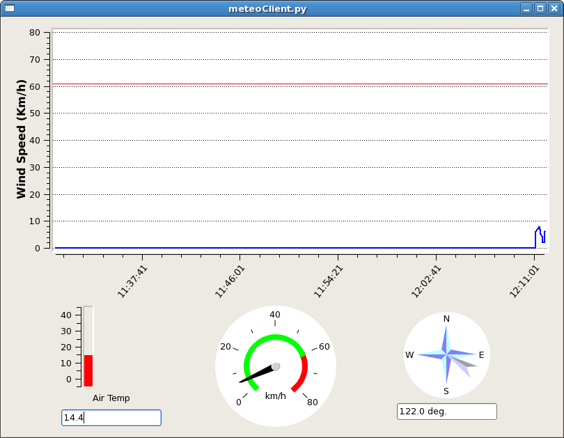
Notice the top graph: the red line corresponds to wind speed = 61 km/h, at which the antenna must be stowed.
Considering that weather parameters are not necessarily written in the output files (in particular, wind speed and direction are not stored in the FITS files at present), it is possible to record a separate log containing these parameters plus information on the antenna pointing. Open a terminal on nuraghe-obs1 and execute the following command:
$ windLogger
The script, besides displaying the information on screen, will produce a file which contains:
coordinates pointed by the antenna;
atmospheric temperature;
wind speed and direction.
These logfiles are stored in a dedicated folder on OBS1:
/archive/logs/WindLog (see also section “Retrieving the data”).
Filenames are assigned according to date and time of the script execution. For example, if the script is launched on November 26th 2013 at 13:46:31 UT, the resulting file will be: azel_131126_134631.log During the acquisition, the shell must not be closed. To interrupt the acquisition, use CTRL+C from the keyboard.
Manual acquisitions
When performing manually commanded acquisitions, it is necessary to select the recording device:
> chooseRecorder=[string]
where string can be:
MANAGEMENT/Point (default) text output in the logfile, used for pointing calibration
MANAGEMENT/CalibrationTool text output in .dat file, used for pointing calibration
MANAGEMENT/FitsZilla if FITS output is desired
(MANAGEMENT/MBFitsWriter) if MBFITS is preferred – not yet available
Note
When recording manually-acquired data in FITS format, the output files are stored in a peculiar path: /archive/extraData. This implies that they also cannot be shown by the quick-look procedure.
Once the recorder is set, acquisitions on a target can be performed as follows. First, set the target:
> track=[sourcename]    (if the source is included in the system
                        catalogue)
For the available catalogue see Appendix D - Source catalogue. To set a generic target:
> sidereal=[sourcename],[RA],[Dec],[epoch],[sector]
(see Antenna operations for details)
Here follow the commands to be used to manually record your data (remember that the backend must have been properly set up and the target must have been specified as explained above):
> initRecording=[scn]
where [scn] in the scan number to be assigned to the acquisition.
The initRecording command prepares the data recording. Then:
> startRecording=[sub_scn],[duration]
creates the output file and begins the data recording; [sub_scn] is the subscan
number, [duration] is the acquisition duration, expressed as hh:mm:ss.
Once the acquisition is completed, the user can launch another subscan and
record the data with another startRecording command.
Finally, once the user wants to close the scan, the command to be used is:
> terminateScan
Output files will be found in the usual auxiliary folder where all the manual acquisitions are destined.
Example: acquisition of a sidereal scan on 3c123 composed by 2 subscans, each lasting 40 s, preceded by an off-source Tsys measurement:
> chooseRecorder=MANAGEMENT/FitsZilla
> track=3c123
> goOff=HOR,5
> waitOnSource
> tsys
> azelOffsets=0.0d,0.0d
> initRecording=1
> startRecording=1,00:00:40
> startRecording=2,00:00:40
> terminateScan
Pointing scans
Command cross-scans across a previously selected target (by means of the track or sidereal commands):
> crossScan=[subscanFrame],[span],[duration]
where subscanFrame is the coordinate frame along which the scan is performed
(eq, hor or gal), span is the spatial length on sky of the
individual subscan (i.e. one line of the cross) expressed in degrees, duration i
s the time length espressed in hh:mm:ss,
e.g.
> crossScan=HOR,1.0d,00:00:30
corresponds to one cross-scan carried out in Horizontal coordinates (one line along El, one line along Az), each line being 1° in span. Each subscan lasts 30 seconds, thus the resulting scan speed is 2°/min.
When the MANAGEMENT/Point writer is used, the cross-scan produces text output in the logfile only (no output file is recorded). This output text contains information obtained by the automatic processing of the subscans. In particular, a Gaussian fit is performed in order to measure the source position and estimate the pointing offsets. If the fitting procedure in successful and the achieved offsets are considered plausible, pointing corrections are immediately applied. This means that, if no user-defined offset is commanded (or cleared) afterwards, the measured offsets remain active and are applied to the following observations.
Here follows the function that is separately fitted to latitude and longitude subscans:
y(x)=A*e^W + ax +c
where:
W = -2.7725887 * F^2
F = (x-μ)/FWHM
μ = abscissa of peak
The results are given in the logfile, in the following sequence of lines:
where (all angles in degrees):
.
Note
it is possible to include such pointing scans using the
MANAGEMENT/Point writer in schedules as well. For example, an improved
pointing can be achieved setting the first scan on a source as a /Point
scan, then – in case the fit is successful – the following scans (e.g.
producing FITS or MBFITS files) will hold the offsets optimising the
pointing, given that no user-defined offset is updated by means of an
explicit radecOffsets, azelOffsets or lonlatOffsets command.
Skydips
Skydip scans are indispensable in order to characterize the atmosphere. They consist in moving the telescope along a vast span in elevation (at fixed azimuth) while sampling with a backend. Their analysis allows the user to quantify the atmospheric opacity τ. There are different ways to perform this:
> skydip=[El1],[El2],[duration]
e.g. skydip=20d,80d,00:05:00 performs a skydip between 80 and 20 degrees
(at the current azimuth position), the scan will take 5 minutes (speed is thus
12 °/min). The arguments must be in the range 10-88.
The jolly character is supported for the elevation arguments.
Example: skydip=*,*,00:04:00 will perfom the skydip between the default
values for elevation (15° and 90°). Please notice that pointing corrections
are disabled.
Since no backend recording is automatically enabled by this command, remember to activate the FitsZilla recorder before launching the command, in order to save the data! This command can be used within schedules as well. See the separate guide to schedules for details.
Note
At present skydips are always performed downwards, i.e. starting from the highest elevation given in the command. The greatest commandable elevation is 88°, since the skydip, being an OTF subscan, will be additioned of an initial acceleration ramp – the length of which is proportional to the scanning speed.
Caveat on offsets
As seen in Antenna operations, there are commands used to set
(or null) user-defined offsets.
They are: radeOffsets, azelOffsets and lonlatOffsets.
Such commands set system offsets which remain active until they are
explicitly changed/nulled by another call of one of the three commands.
Further offsets, having for example the purpose of pointing the antenna to an off-source position, are specified inside schedules, at the subscan level (see the separate guide to schedules). The subscan-level offsets sum up to the overall offsets if they are expressed in the same coordinate frame, and they are zeroed by default every time a new subscan is commanded.